Why Your Spatial Transcriptomics Analysis Might Be Lying to You (I)

So here’s the thing about analyzing gene expression data. You load up your Xenium or Visium dataset, you run the standard Seurat or SpatialData pipelines because that’s what everyone does, you get your clusters, and you write your paper. Great. Except maybe not great, because it turns out that the normalization step you copied from the single-cell RNA-seq tutorial might be quietly removing the very biological signal you’re trying to find.

This isn’t hypothetical hand-waving. Data from recent benchmarking studies tells a pretty clear story. When you apply standard single-cell normalization methods to spatial transcriptomics data, especially in tissues with anatomically structured variation in cell density or RNA content, you can inadvertently erase genuine biology. The cortical white matter doesn’t have uniform cell packing. The liver lobule has zones with different metabolic activities and different RNA abundances. These regional differences aren’t technical noise, they’re the biology. But if you normalize them away, they’re gone.

Let’s unpack how we got here and what we can do about it.

The Normalization Problem: What We’re Actually Trying to Fix

Single-cell RNA sequencing generates count matrices where each number represents detected mRNA molecules. The raw count for any gene in any cell reflects true expression plus a whole stack of technical artifacts. Cell lysis efficiency varies. mRNA capture rates fluctuate. Amplification introduces biases. Sequencing depth differs across cells. These technical factors create cell-specific and gene-specific effects that confound biological interpretation if you don’t correct for them.

The standard approach has been to compute some kind of size factor per cell and scale everything uniformly. LogNormalize in Seurat does exactly this. It divides each gene’s count by the total counts in that cell, multiplies by 10,000, and takes the log. The math is simple: log(count/total × 10000 + 1). The assumption is also simple: all genes scale uniformly with sequencing depth. This assumption works reasonably well for identifying cell types in peripheral blood mononuclear cells or dissociated tissues where cells are randomly distributed.

Here’s where spatial data breaks that assumption. In spatial transcriptomics, cells aren’t randomly distributed. They’re organized into anatomical structures with systematic differences in cell density, cell types, and transcriptional activity. The white matter has fewer cells than gray matter. The portal zone of the liver lobule has different metabolic demands than the central vein region. These spatial gradients in total RNA content aren’t technical artifacts, they’re biology. When you normalize by total counts per spot or per cell, you’re assuming that variation in library size is purely technical. But what if it’s not?

From Simple Scaling to Statistical Frameworks

The field has evolved from these simple scaling approaches toward methods that model the statistical properties of count data more carefully. I’ll walk through the major categories because understanding the underlying logic matters more than memorizing method names.

Global scaling methods like LogNormalize, CPM (counts per million), and TPM (transcripts per million) compute a single size factor per cell and scale all counts uniformly. These work fine when the assumption holds that library size variation is mostly technical. TPM adds gene length correction, which matters for full-length protocols but not for 3’ end counting methods where one transcript generates one count regardless of length.

Pooling-based methods like scran take a different approach. Instead of computing size factors from individual cells, which fails when cells have lots of zeros, scran aggregates counts across pools of similar cells. This overcomes zero inflation by working with more robust pool-level totals before deconvolving back to cell-level factors. The method explicitly addresses the dropout problem where expressed transcripts fail to be captured.

Regression-based methods model count data using generalized linear models with sequencing depth as a covariate. SCTransform represents the most widely adopted approach in this category. It fits a regularized negative binomial regression for each gene, modeling the mean-variance relationship and stabilizing variance across expression levels. The second version (SCTransform v2) improves handling of datasets with different sequencing depths across conditions, which reduces false positives in differential expression analysis.

Bayesian methods like BASiCS and SCDE use probabilistic frameworks to separate technical from biological variation. These approaches model dropout events explicitly and can distinguish biological zeros from technical failures. The trade-off is computational cost, which scales poorly to large datasets.

Deep learning methods like scVI use variational autoencoders to learn low-dimensional representations while accounting for technical noise. The model learns to disentangle biological variation from batch effects and library size effects without requiring explicit statistical assumptions about the count distribution. These methods work particularly well for integration tasks where you’re combining multiple datasets.

Count-preserving methods represent an alternative philosophy. Instead of transforming counts through normalization, methods like countland work directly with integer counts using models that naturally handle count data. This preserves the discrete nature of molecular counting and avoids potential artifacts from log transformations.

Each approach makes different assumptions about the data generating process. No single method wins across all contexts.

What Works for Single-Cell RNA-seq

Benchmarking studies have evaluated these methods across diverse datasets and analytical tasks. For standard single-cell RNA-seq analysis, particularly with UMI-based protocols like 10x Genomics, current best practices converge on a few options.

SCTransform v2 performs well for clustering and differential expression, especially when comparing conditions with different sequencing depths. The variance stabilization it provides reduces the impact of mean-variance relationships that can create spurious patterns. Scran remains a solid choice, particularly for integration workflows where it’s been extensively validated. Recent work suggests Dino, which models the full distribution of counts for variance stabilization, performs particularly well for high-throughput clustering applications.

The key insight is that method choice depends on experimental context and analytical goals. Full-length protocols like Smart-seq2 benefit from gene length normalization that’s irrelevant for UMI data. Integration tasks may favor deep learning approaches that can handle complex batch structures. Differential expression testing requires methods that control false positive rates appropriately.

Where Spatial Data Breaks the Rules

Spatial transcriptomics introduces a fundamental complication. The spatial association between region-specific library size and underlying biology means that standard normalization can remove genuine signal.

Consider a Visium experiment profiling brain tissue. Cortical white matter has lower cell density and lower total RNA content than gray matter. This creates a spatial gradient in library size that corresponds to anatomical structure. If you apply standard LogNormalize, you’re implicitly treating this gradient as technical noise and normalizing it away. But the gradient is biology. Different brain regions have different cellular compositions and different transcriptional programs.

This problem becomes even more acute with subcellular resolution platforms like Xenium or CosMx. Individual cells have spatial organization of organelles, transcripts localize to specific subcellular compartments, and RNA abundance varies systematically across cellular domains. Normalizing by cell-level totals can obscure these patterns.

Recent work from Svensson and colleagues demonstrated this problem empirically. They showed that applying standard single-cell normalization methods to spatial data can reduce performance in spatial domain identification tasks. In some datasets, unnormalized or minimally normalized data (just log transformation) outperformed aggressively normalized data for identifying anatomical regions.

The issue is that we borrowed tools designed for one problem (technical variation in dissociated single cells) and applied them to a different problem (spatial biology where location matters). The assumptions don’t transfer cleanly.

Practical Recommendations: What to Actually Do

When analyzing spatial transcriptomics data, start by examining the raw data. Plot spatial distributions of total counts and key marker genes. Look for regional patterns. If you see systematic spatial variation that corresponds to known anatomical structures, be cautious about aggressive normalization.

For spatial domain identification, consider minimal normalization or log transformation without scaling. Recent benchmarks suggest this often works better than methods that remove spatial library size variation.

If you use standard methods like LogNormalize, validate your results against known biology. Marker genes with established spatial patterns provide internal validation. If your normalized data shows uniform expression of a gene that should be spatially restricted, your normalization likely removed signal.

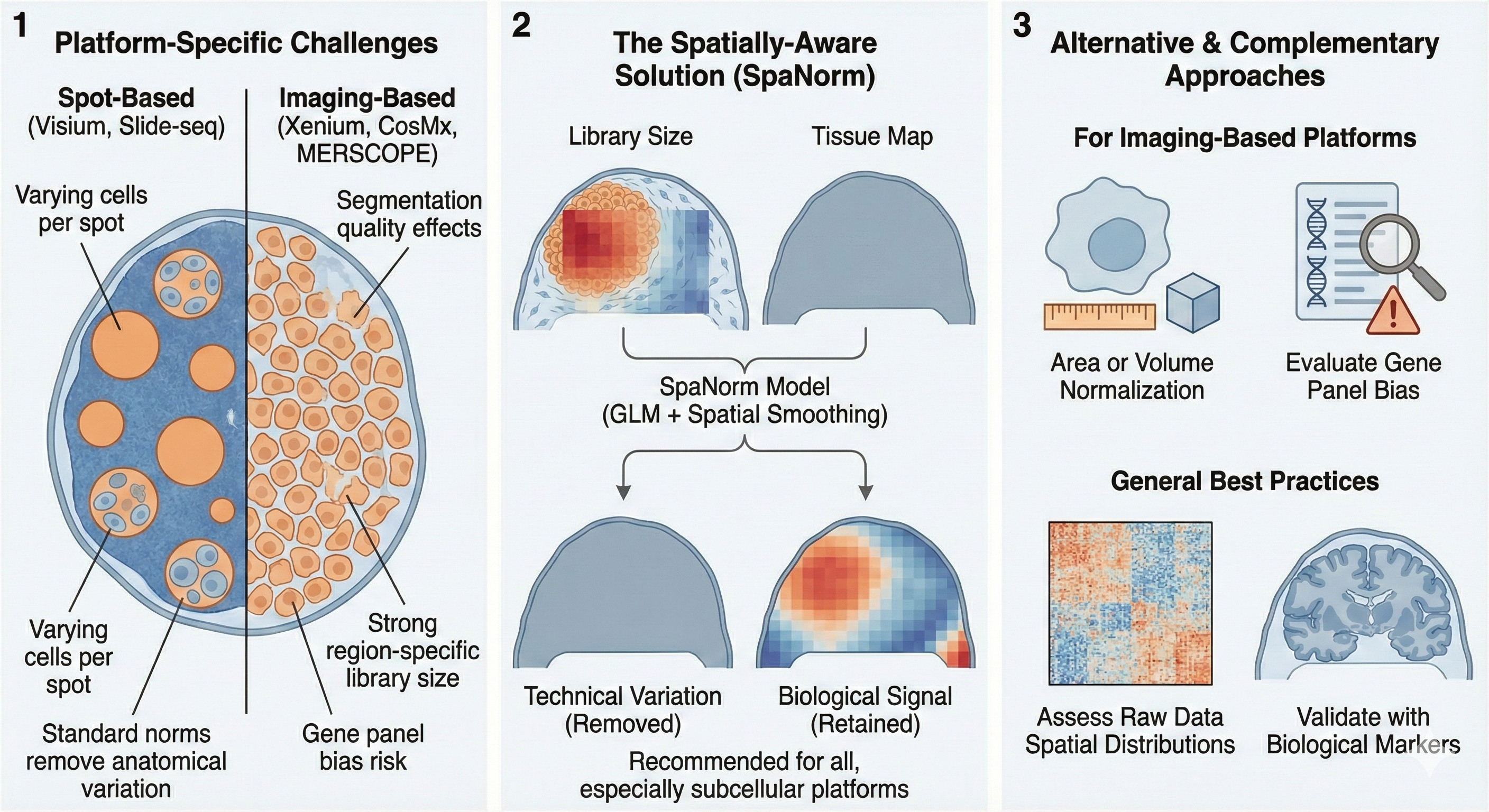
For imaging-based platforms with defined gene panels, evaluate whether the panel composition introduces systematic biases. Consider area-based or volume-based normalization as alternatives to count-based methods, particularly for subcellular resolution data.

SpaNorm provides a purpose-built solution for data where spatial library size variation reflects biology. The method is most valuable for tissues with strong anatomical organization and for subcellular resolution platforms.

For differential expression analysis in spatial data, pseudobulk approaches that aggregate spots within regions and apply bulk methods remain a robust choice. This sidesteps many normalization challenges by working at the region level rather than spot level.

The Deeper Issue: Technical Noise Versus Biological Signal

The normalization problem in spatial transcriptomics highlights a broader challenge in computational biology. We build tools to remove technical variation, but those tools encode assumptions about what counts as technical versus biological. When data structure violates those assumptions, our corrections become overcorrections.

This matters because spatial transcriptomics is moving toward higher resolution, greater multiplexing, and multimodal integration. Subcellular resolution platforms let us see transcript localization patterns. Multiplexed imaging adds protein measurements. These technologies generate data where spatial structure carries biological information that we need to preserve.

The solution isn’t to abandon normalization. Raw count data has real technical artifacts that need correction. The solution is to develop methods that respect spatial structure while removing noise. SpaNorm represents a first step. Methods that incorporate tissue architecture, cell type composition, and spatial autocorrelation will likely follow.

For multimodal data combining RNA and protein measurements, we need modality-specific approaches. Protein data from CITE-seq experiments shows different statistical properties than RNA counts. Methods like CLR (centered log ratio) and dsb explicitly address antibody-derived protein data characteristics. As technologies integrate more data types, normalization strategies will need corresponding sophistication.

What This Means for Your Analysis

If you’re analyzing spatial transcriptomics data, the default pipeline might not be your friend. The standard workflow that works beautifully for PBMC single-cell data can quietly remove spatial biology from tissue data.

Before normalizing, understand what your method assumes. LogNormalize assumes uniform scaling relationships. SCTransform assumes mean-variance relationships follow a specific form. Deep learning methods make implicit assumptions through their architecture choices. If your data violates these assumptions, your normalization will distort your results.

Validate against known biology. If you have marker genes with established spatial patterns, check that your normalized data preserves those patterns. If normalization removes them, you’ve overcorrected.

Consider whether you need normalization for your specific analysis. For some spatial domain identification tasks, minimal processing works better than aggressive normalization. For differential expression, pseudobulk approaches offer robustness. For integration, spatially-aware methods matter.

The fundamental goal remains unchanged: distinguish technical variation from biological variation while preserving the latter. But in spatial data, where spatial variation is often biological, we need tools that respect that structure.

Looking Forward

The field is moving fast. Spatial transcriptomics technologies continue to improve in resolution and throughput. Normalization methods are adapting accordingly. Spatially-aware approaches will become more sophisticated as we better understand tissue architecture and spatial gene expression patterns.

Integration of multiple data modalities will require normalization methods that handle RNA, protein, metabolites, and morphological features simultaneously. Each modality has different noise characteristics and different scaling relationships.

Machine learning approaches will likely play an increasing role. Methods that learn normalization strategies from data rather than imposing parametric assumptions could adapt to diverse experimental contexts. The challenge will be maintaining interpretability and biological validity.

For now, the practical advice is simple. Understand your tools. Validate your results. Don’t assume that methods designed for single-cell RNA-seq transfer directly to spatial data. The biology is different, the technical artifacts are different, and the normalization strategy should be different too.

Your spatial transcriptomics data contains rich biological information about tissue organization, cellular interactions, and spatial gene expression patterns. Choose normalization methods that preserve that information rather than normalize it away.